
I’m not sure how old I was when I first created a cellular automata. I suspect in my early teens, sat in front of a BBC Micro typing in the Basic code for Conway’s Life from a magazine. At the time I was more interested in coding fractals and the Mandelbrot set. My imagination was not gripped.
While doing my M.Sc. in computer science I produced a graphical program for running various cellular automata in my final dissertation. The focus at the time was much more on the “computer” rather than the “science”. Beyond replicating well know rules I did little to advance my understanding of these simple little programs.
Fast forward a few decades. I’m watching the family play Minecraft, which on some levels can be mistaken for one large 3D automata. I’m reading about complexity in pretty much any management book I pick up. At work I’m seeing strange behaviour in the infrastructure of complex enterprise systems. I’ve also started coding again. It was enough to rekindle my interest in the subject.
I begin by purchasing the beautifully illustrated book, A New Kind of Science, by Stephen Wolfram (published in 2002). I’ll be using some of Wolfram’s notation for convenience. However please don’t take that as a recommendation it is a controversial book for good reason.
The most basic cellular automata used by Wolfram takes 3 inputs. Each cell uses its own state and that of the two nearest neighbour’s to calculate it’s next state. My initial thought is that it may be possible to start with a rule which only requires 2 inputs. This simplification has the added benefit of allowing rules to be described in the language of logic gates e.g. AND, NAND, OR, XOR etc. The diagram below illustrates the point and shows 3 possible configurations for our logic gates.

The table below lists the 16 possible rules for the 2 input automata. Each is translate into the equivalent Wolfram rule numbers. Note each configuration can result in a different Wolfram rule number. Where applicable a logic gate name has also been given.
| Rule No. | Left + Self | Left+Right | Self+Right | Logic Gate |
|---|---|---|---|---|
| 0 | 0 | 0 | 0 | |
| 1 | 3 | 5 | 17 | NOR |
| 2 | 12 | 10 | 34 | |
| 3 | 15 | 15 | 51 | |
| 4 | 48 | 80 | 68 | |
| 5 | 51 | 85 | 85 | |
| 6 | 60 | 90 | 102 | XOR |
| 7 | 63 | 95 | 119 | NAND |
| 8 | 192 | 160 | 136 | AND |
| 9 | 195 | 165 | 153 | XNOR |
| 10 | 204 | 170 | 170 | |
| 11 | 207 | 175 | 187 | |
| 12 | 240 | 240 | 204 | |
| 13 | 243 | 245 | 221 | |
| 14 | 252 | 250 | 238 | OR |
| 15 | 255 | 255 | 255 |
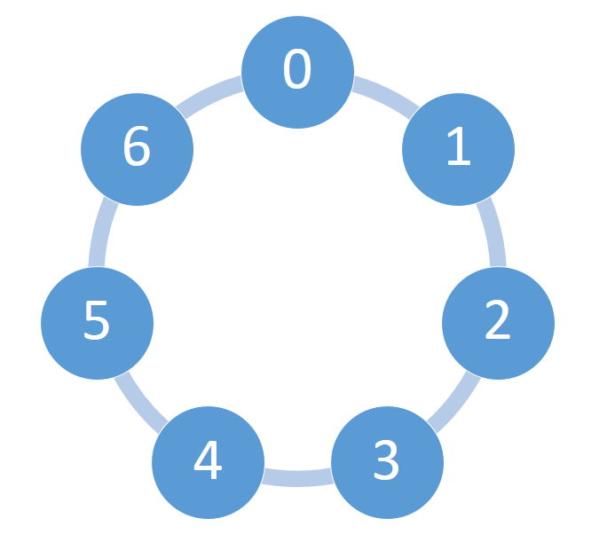
The next simplification is to constrain the space available to the simple 2 dimensional cellular automata. Infinite space means growth can be unbounded. The simplest bounded space is made by joining together the two ends of the line. An example 7 cell universe is shown in the diagram below. Cell zero is now neighbours with cell six.
Constraining the space available to the automata has an effect on limiting the complexity. In the example size 7 space, this gives us 128 possible states. The question now is, with the reduction of inputs from 3 to 2 and with a finite number of states, can we still see aspects of complex and chaotic behaviour? Perhaps not something I’ll be able to answer one way or another in a single blog post.
Before looking for signs of complexity let’s begin with the basic behaviour of our mini-universe. Below is shown Rule 90 being applied to a size 7 space. The space is seeded with a single cell with value 1. There appears to be a short period of rapid expansion. It takes 3 ticks of our automata’s clock to reach the boundaries. After that the rule settles into a repeating pattern which takes 7 ticks to play out, after this point the model is stable. Beyond this point there are no more surprises. A sure sign we’ve left the realms of chaos and complexity.

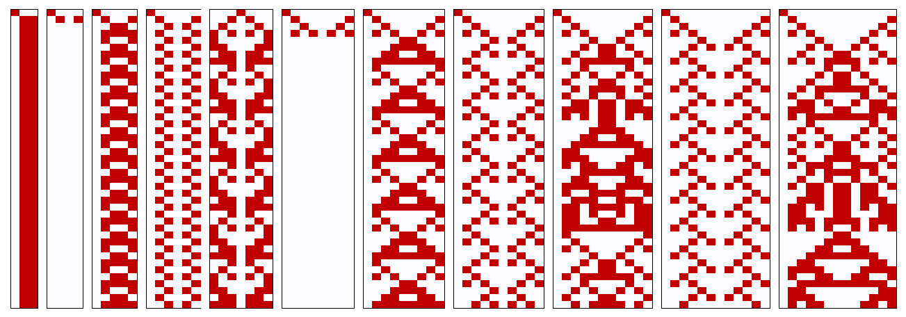
I’ve rushed ahead a little. By selecting Rule 90 I have settled on one of the more interesting patterns. So backing up slightly here are all the patterns produced in our simple 7 cell universe. Notice how 9, 11, 13, and 15 are negative images of other rules. While 4,5,12 are mirror images. There is also some duplication with 8 and 10.

At this stage with a simple one cell seed, this leaves us with Rule 90 (No. 6) looking the most interesting so let’s see how that varies with size of space.
So at first look it appears under certain conditions we are able to produce complex looking patterns at certain sizes (7, 11, 13) and using nothing more than XOR logic gates. Given this starting point next I’ll do a more thorough analysis of the variations, however that will have to wait for another post.


